Septoria on wheat in Indiana • FraNchEstYN

🎯 Goal

This vignette walks through the process of fitting Septoria tritici blotch severity data in Indiana using FraNchEstYN. We will use the example datasets bundled with the package:

weather_indiana: daily weather data (NASA POWER)
reference_indiana: digitized disease observations from Shaner & Buechley (1995)
management_indiana: sowing and crop management metadata from the same article.

📦 Packages

We load the FraNchEstYN package plus some helper libraries for data handling, tables, and plotting.

library(FraNchEstYN) 
library(tidyverse)
library(kableExtra)
library(plotly)

📥 Data loading

The three Indiana datasets are included with the package. Below we load them and preview a few rows to illustrate their structure.

data(weather_indiana)
data(reference_indiana)
data(management_indiana)

weather_indiana — daily weather (first rows)
site	year	month	day	tx	tn	p	rad
Indiana	1972	1	1	6.623	-2.085	0.000000	7.45
Indiana	1972	1	2	2.450	-3.212	3.313559	9.44
Indiana	1972	1	3	5.360	-2.956	0.000000	8.31

reference_indiana — disease observations
site	year	DOY	FINT	Disease
Indiana	1973	144	1.00	NA
Indiana	1973	187	0.25	NA
Indiana	1974	141	1.00	NA

management_indiana — management metadata (first 6 rows)
site	crop	variety	year	sowingDOY
Indiana	wheat	Generic	1972	278
Indiana	wheat	Generic	1973	271
Indiana	wheat	Generic	1974	275

⚙️ Parameters

In FraNchEstYN, crop and disease processes are controlled by parameter sets referred to physiological and epidemiological traits.

In this vignette we are only interested in canopy light interception and disease severity, not yield formation.

For wheat: start from defaults, disable calibration of traits unrelated to light interception, and keep canopy dynamics active.
For Septoria: start from defaults, and disable calibration of yield-loss damage mechanisms. Therefore, we:

# Load default parameters for wheat
thisCropParam <- cropParameters$wheat

# Disable all calibration, then selectively re-enable light interception
thisCropParam <- set_calibration_flags(
  thisCropParam,
  disable = c("PartitioningMaximum",
              "TbaseCrop", "TmaxCrop", "ToptCrop",
              "FloweringStart",
              "RadiationUseEfficiency")
)

# Load default parameters for Septoria
thisDiseaseParam <- diseaseParameters$septoria

# Disable calibration for yield-loss damage mechanisms
thisDiseaseParam <- set_calibration_flags(
  thisDiseaseParam,
  disable = c("RUEreducerDamage",
              "LightStealerDamage",
              "SenescenceAcceleratorDamage",
              "AssimilateSappersDamage")
)

🔧 Calibration model call

With data and parameters prepared, we can call the FraNchEstYN calibration engine. Here we fit both crop and disease model parameters simultaneously, using the Indiana datasets.

Key settings: - start_end: simulation period (1971–1992 in this example)
- api_key: required for external API calls, but not used here
- franchy_message: set to FALSE to silence fun messages 😉
- iterations: number of optimization iterations (666 here, the devil’s number 👹)
- calibration: scope of calibration ("all" means crop + disease)

This returns a model object df containing diagnostics, parameters, and simulation outputs.

start_end <- c(1971, 1992)
api_key <- "xxx"         # not used here for LLM
franchy_message <- FALSE
iterations <- 100        # the more iterations, the longer it takes but results are safer
calibration <- "all"     # calibrate both crop and disease

df <- franchestyn(
  weather_data      = weather_indiana,
  management_data   = management_indiana,
  reference_data    = reference_indiana,
  cropParameters    = thisCropParam,
  diseaseParameters = thisDiseaseParam,
  start_end         = start_end,
  calibration       = calibration,
  apikey            = api_key,
  franchy_message   = franchy_message,
  iterations        = iterations
)

📊 Outputs & results

⚖️ Parameter plots

Plots show parameter ranges, defaults, and calibrated values:

Black / grey lines = allowable parameter ranges
🔵 Blue vertical line = default value
🔴 Red dot = calibrated value (if calibration was enabled)

Note: crop parameters here remain at defaults (blue line only), while disease parameters include calibrated values.

df$diagnostics$calibration$plots$crop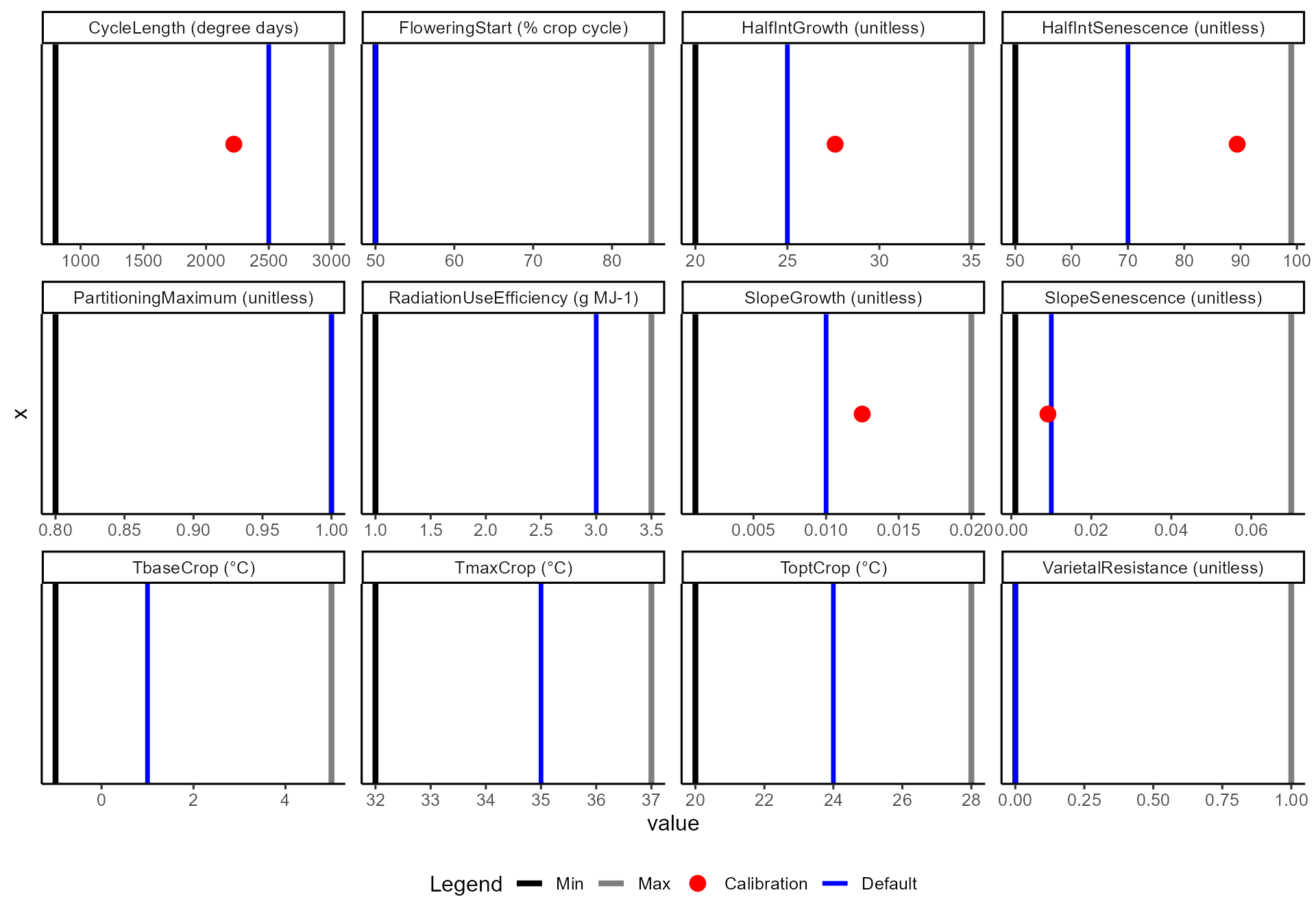

df$diagnostics$calibration$plots$disease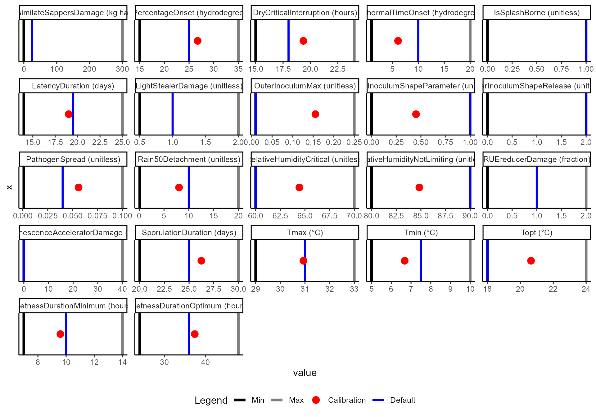

📏 Calibration metrics (Disease Severity)

We summarise calibration accuracy for disease severity across seasons using Bias, MAE, RMSE, correlation, R², and NSE.

Calibration metrics for disease severity (DisSev)
GrowingSeason	n	Bias	MAE	RMSE	r	R2	NSE
1972	8	-0.125	0.127	0.151	0.960	0.922	0.752
1973	8	0.136	0.229	0.248	0.866	0.750	0.486
1974	6	-0.139	0.139	0.157	0.980	0.960	0.426
1975	9	0.122	0.187	0.210	0.846	0.716	0.503
1976	3	-0.025	0.148	0.175	0.842	0.709	0.371
1977	5	0.000	0.068	0.079	0.893	0.798	0.599
1978	6	0.105	0.179	0.197	0.758	0.575	0.375
1979	6	0.009	0.077	0.106	0.950	0.903	0.875
1980	8	-0.141	0.141	0.151	0.984	0.968	0.701
1981	4	0.109	0.146	0.163	0.926	0.857	0.627
1982	7	-0.005	0.033	0.038	0.991	0.982	0.975
1983	4	0.110	0.110	0.120	0.948	0.899	0.012
1984	2	0.255	0.255	0.277	1.000	1.000	-25.046
1985	5	0.054	0.210	0.228	0.909	0.826	0.564
1986	5	-0.287	0.287	0.363	0.801	0.642	-1.091
1987	4	-0.010	0.010	0.011	0.988	0.976	0.899
1988	8	-0.115	0.115	0.172	0.987	0.973	0.699
1989	7	-0.098	0.106	0.129	0.948	0.899	0.762
1990	5	0.064	0.209	0.220	0.868	0.754	0.475

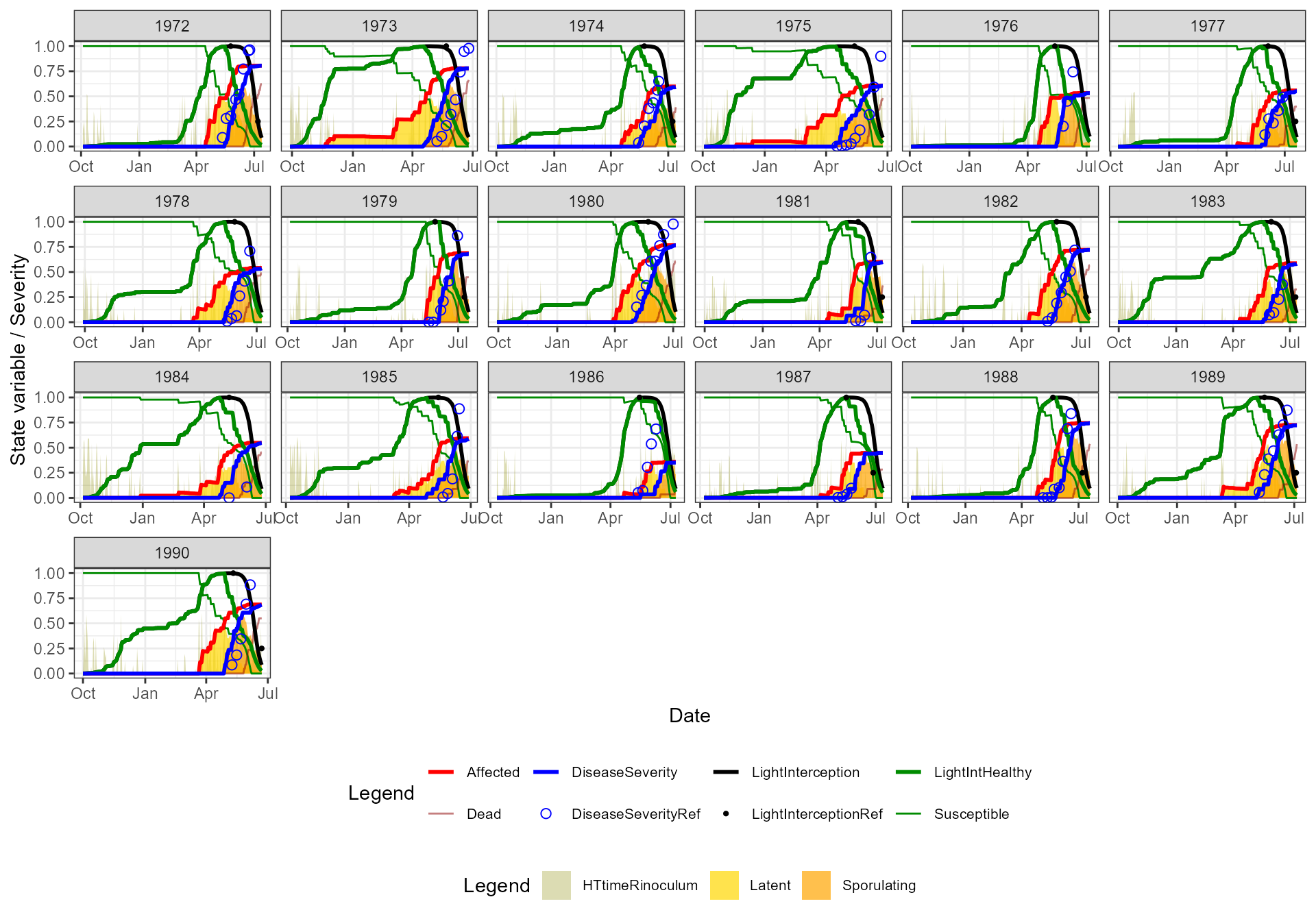
📈 Simulation outputs

🗂️ Season summary

A compact table of disease severity outcomes for each growing season: final severity, peak, timing, and area-under-curve.

summary of simulated disease severity
GrowingSeason	Site	AveTx	AveTn	AveRHx	AveRHn	TotalPrec	TotalRad	TotalLW	AUDPC	DiseaseSeverity
1972	Indiana	12.414	4.065	80.582	48.308	875.504	3652.87	1917	3205.647	0.806
1973	Indiana	12.563	3.384	79.394	45.080	1012.792	3353.07	2160	3289.634	0.779
1974	Indiana	12.618	3.895	79.092	45.908	737.493	3922.62	1659	2163.079	0.593
1975	Indiana	13.385	3.172	78.092	41.581	569.914	3732.22	1402	2669.848	0.606
1976	Indiana	11.557	1.868	72.148	39.199	575.648	4027.05	1164	2239.769	0.531
1977	Indiana	10.699	1.379	70.966	39.693	668.018	3996.45	1527	2059.912	0.550
1978	Indiana	11.516	2.033	74.625	40.793	742.898	3871.05	1714	2372.080	0.537
1979	Indiana	12.410	3.371	77.502	43.676	817.637	3898.40	1528	2468.710	0.679
1980	Indiana	12.373	3.007	77.890	43.696	856.521	3790.90	1564	3056.156	0.766
1981	Indiana	11.367	1.718	73.992	40.617	865.298	3948.87	1820	1903.726	0.600
1982	Indiana	13.263	4.501	81.318	47.267	832.473	3699.41	1582	2941.946	0.720
1983	Indiana	11.415	2.658	75.902	43.926	832.008	3759.49	1733	1980.241	0.582
1984	Indiana	12.454	3.222	78.083	43.808	956.927	3410.67	1722	2190.895	0.548
1985	Indiana	12.504	3.297	77.475	44.170	839.796	3386.69	1613	1980.329	0.587
1986	Indiana	13.415	4.321	78.867	44.761	576.309	3787.24	1211	934.490	0.351
1987	Indiana	13.535	3.427	75.746	40.274	596.667	4248.61	1201	1810.863	0.447
1988	Indiana	12.894	3.498	78.834	43.313	843.670	4116.81	1687	2735.966	0.745
1989	Indiana	12.774	3.598	79.528	44.815	737.459	3684.23	1493	2677.643	0.722
1990	Indiana	13.693	4.171	79.760	43.890	766.784	3458.94	1604	2736.972	0.685

🗺️️ Multi-season overview (static)

Facetted plots across seasons showing dynamics of inoculum, latent and sporulating tissue, canopy light interception, and disease severity vs. observations.

🎯 1972 deep-dive (interactive)

An interactive plot of the 1972 season lets us hover over state variables and observed values.

📝 Key take-home messages

FraNchEstYN successfully calibrated disease severity for Septoria tritici in Indiana across two decades of observations.
Crop parameters were mostly fixed (default values) — only canopy light interception was active, while disease parameters were calibrated.
The framework provides diagnostics, metrics, parameter estimates, and simulations in a consistent structure, ready for analysis or visualization.

🚀 Next steps

This vignette showed how to calibrate Septoria tritici blotch severity in Indiana using bundled datasets. From here, you might want to:

🌎 Explore other environments: replace weather_indiana, reference_indiana, and management_indiana with datasets from different sites or years.

🌾 Switch crops or pathogens: try other parameter sets available in cropParameters and diseaseParameters.

🎛️ Experiment with calibration scope:

“all” → calibrate both crop and disease models

“crop” or “disease” → focus on one component only

📊 Analyze uncertainty: increase the number of iterations or run multiple calibration replicates to assess stability of parameter estimates.

🛠️ Extend the pipeline: integrate with your own management practices or link outputs to yield-loss models. .